You don’t need a political pundit to tell you what your eyes, ears and presidential primary results show – in 2016 the electorate is angry. The economy isn’t at the top of every voters mind in every election but it is close. For decades nearly every presidential candidate from both incumbent and non-incumbent political parties has asked voters “are you better off today than you were four years ago?” As I documented in one of the very first posts in this blog, when the majority response was “yes,” the incumbent party’s candidate was almost certain to capture the White House. There are some troubling economic trends and vexing economic issues affecting large numbers of Americans, still, to me the apparent level of anger in the electorate today seems outsized in historical context.
By most aggregate measures the country, as well as most individual states, are better off economically today than in 2012. The simple calculus of Arthur Okun’s “misery index” – or the combined rates of unemployment and inflation – long a shorthand metric for assessing the likely aggregate economic sentiment of the American electorate, is much lower today than it was in 2012 suggesting that, collectively at least, we should feel somewhat better off. But the level of anger in political and public discourse has elevated during the past four years and the old “misery index” now seems a woefully inadequate measure of the electorate’s assessment of current economic conditions.
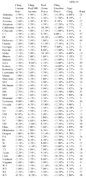
Adding economic variables that have a demonstrable impact on American’s perceptions of the economy to the “misery index” – such as gasoline prices, home price appreciation, and household income – only adds to the apparent disconnect between standard economic metrics and current voter sentiment. The table below shows, on a percentage basis, how much lower is the unemployment rate (since 2012), how much real household personal income has grown (since 2013), how much real home price appreciation has occurred in the past two years, and how much lower are gasoline prices over the last year, in each of the 50 states. In addition, the table assigns weights (subjective though they may be) to the income, home price, and gasoline price measures to develop an aggregate measure of how much better or worse off the electorate is in each state over the past several years. (The unemployment rate is not included in the combined metric because it is already captured as a determinant of changes in real household personal income).
 Misery metrics aside, historical election results show that regardless of economic conditions there is a tendency for many states to vote consistently for the candidate from one political party (the Democratic candidate has not garnered even 40% of the presidential vote since 1964 in Wyoming and the Republican candidate has won a majority in Massachusetts only once in the past 60 years). In addition, there is clear evidence of ‘voter fatigue” with the incumbent party after two terms in the White House that, depending on the state, can reduce the percentage of the incumbent party’s vote total by as much as 5%. All of this makes me question the value of economic metrics in predicting presidential elections – just not enough to overcome my left brain obsession with developing quantitative analytical models to explain all things. I am no political pundit and this is an economics and policy blog not a political blog – this post has nothing to do with arguing for one presidential candidate or one party over another.
I examined the statistical relationship between voting patterns and key economic variables and used the relationships between non-economic variables (voter fatigue, current presidential approval ratings, etc.) found by others to estimate the percentage of the vote that both the Republican and Democratic candidate would receive in each state and to produce the electoral vote totals in the two graphics below. The model is based on the most recent economic and other data and does not take into consideration the quality or characteristics of the potential candidates – a significant shortcoming as in this election in particular, who the candidates are would seem to have a large impact.

The first graphic (or base scenario) suggests an election that should be reasonably close but with a victory for the Democratic candidate. The second graphic shows a much larger margin of victory for the Democratic candidate. The only difference between the two scenarios is in the importance (statistical coefficient) of the voting trend variable. Each state exhibits a different strength of voting trend (for one party or the other) but after the time needed to statistically determine the trend variable in several states I opted to examine an easier, cross sectional, 50 state aggregate trend variable. This is a sub-optimal solution because the trend variable has a large impact on results.

In the first chart the voting trend variable has a somewhat weaker impact on the vote percentages, while the second chart shows a somewhat stronger impact than I found in my cross sectional analysis. Each chart also shows states that are most likely to switch from either a Democratic (light blue) or Republican (light red) win.
I make no claim that this analysis will bear any relationship to actual election results and this post should make clear why I should stick to policy and not politics, but it has been an interesting exercise in examining the impact of the economy on elections and I will update the charts in the coming months to see how key variables impact the predictions.